Part 3: Working with large-scale data

Intro to Computational Studies in Education and the Social Sciences

Nathan Alexander, PhD

School of Education

Center for Applied Data Science and Analytics

Case Study: HBCUs and Educational Geography

In this section, we analyze data on Historically Black Colleges and Universities (HBCUs) to explore patterns in location, institutional type, and founding history.

Step 1: Load Packages

#install.packages("tidyverse")
#install.packages("lubridate")
library(tidyverse)
library(lubridate)

We’ll start with a guided example using data on Historically Black Colleges and Universities.

Step 2: Load the data

library(tidyverse)
hbcu <- read_csv("https://raw.githubusercontent.com/quant-shop/intro-comp-educ-soc/refs/heads/main/data/hbcu_data.csv")

# View the first few rows
head(hbcu)

# A tibble: 6 × 7
  name                     city       state founded   lat   lon type           
  <chr>                    <chr>      <chr>   <dbl> <dbl> <dbl> <chr>          
1 Alabama A&M University   Normal     AL       1875  34.8 -86.6 Public, 4 Year 
2 Alabama State University Montgomery AL       1867  32.4 -86.3 Public, 4 Year 
3 Albany State University  Albany     GA       1903  31.6 -84.2 Public, 4 Year 
4 Alcorn State University  Lorman     MS       1871  31.9 -91.1 Public, 4 Year 
5 Allen University         Columbia   SC       1870  34.0 -81.0 Private, 4 Year
6 American Baptist College Nashville  TN       1924  36.2 -86.8 Private, 4 Year

# Check structure
glimpse(hbcu)

Rows: 102
Columns: 7
$ name    <chr> "Alabama A&M University", "Alabama State University", "Albany …
$ city    <chr> "Normal", "Montgomery", "Albany", "Lorman", "Columbia", "Nashv…
$ state   <chr> "AL", "AL", "GA", "MS", "SC", "TN", "AR", "SC", "NC", "FL", "A…
$ founded <dbl> 1875, 1867, 1903, 1871, 1870, 1924, 1884, 1870, 1873, 1904, 19…
$ lat     <dbl> 34.7834, 32.3643, 31.5785, 31.8769, 34.0298, 36.1659, 34.7465,…
$ lon     <dbl> -86.5683, -86.2952, -84.1543, -91.1458, -81.0115, -86.7844, -9…
$ type    <chr> "Public, 4 Year", "Public, 4 Year", "Public, 4 Year", "Public,…

# Summary statistics
summary(hbcu)

     name               city              state              founded    
 Length:102         Length:102         Length:102         Min.   :1837  
 Class :character   Class :character   Class :character   1st Qu.:1870  
 Mode  :character   Mode  :character   Mode  :character   Median :1886  
                                                          Mean   :1895  
                                                          3rd Qu.:1905  
                                                          Max.   :1988  
      lat             lon             type          
 Min.   :18.34   Min.   :-98.50   Length:102        
 1st Qu.:32.48   1st Qu.:-90.13   Class :character  
 Median :34.02   Median :-84.64   Mode  :character  
 Mean   :34.31   Mean   :-85.13                     
 3rd Qu.:36.17   3rd Qu.:-80.78                     
 Max.   :39.93   Max.   :-64.96                     

Step 3: Clean the data

hbcu <- hbcu %>%
  mutate(
    founded = as.numeric(founded),
    type = as.factor(type),
    state = as.factor(state)
  )

Step 4: Basic Exploration

How many institutions are in the data set?

nrow(hbcu)

[1] 102

What is the distribution by HBCU type?

hbcu %>%
  count(type) %>%
  arrange(desc(n))

# A tibble: 5 × 2
  type                     n
  <fct>                <int>
1 Private, 4 Year         45
2 Public, 4 Year          40
3 Public, 2 Year          11
4 Private, Specialized     4
5 Private, 2 Year          2

Step 5: Historical Analysis

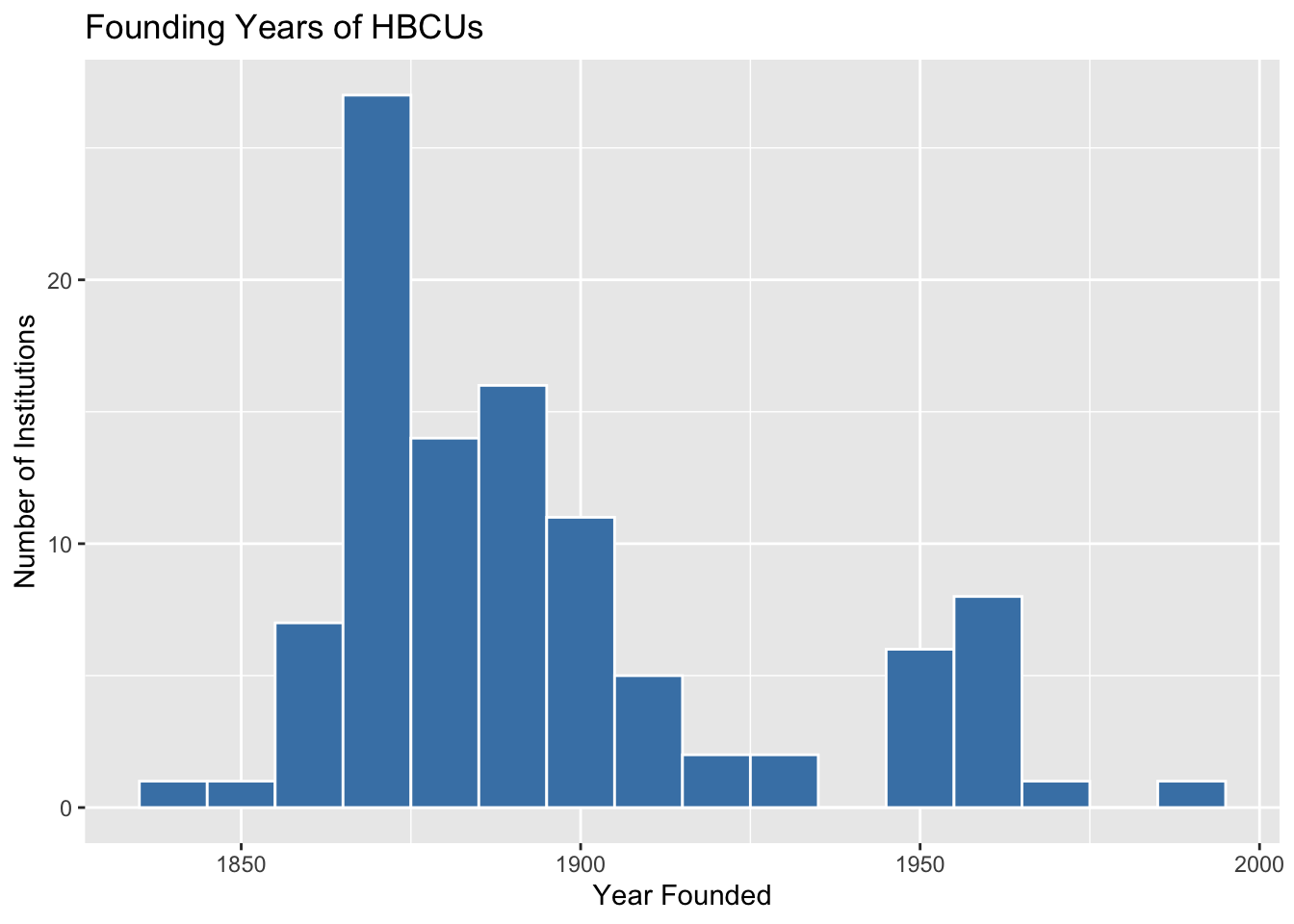
When were the HBCUs founded?

hbcu %>%
  ggplot(aes(x = founded)) +
  geom_histogram(binwidth = 10, fill = "steelblue", color = "white") +
  labs(
    title = "Founding Years of HBCUs",
    x = "Year Founded",
    y = "Number of Institutions"
  )

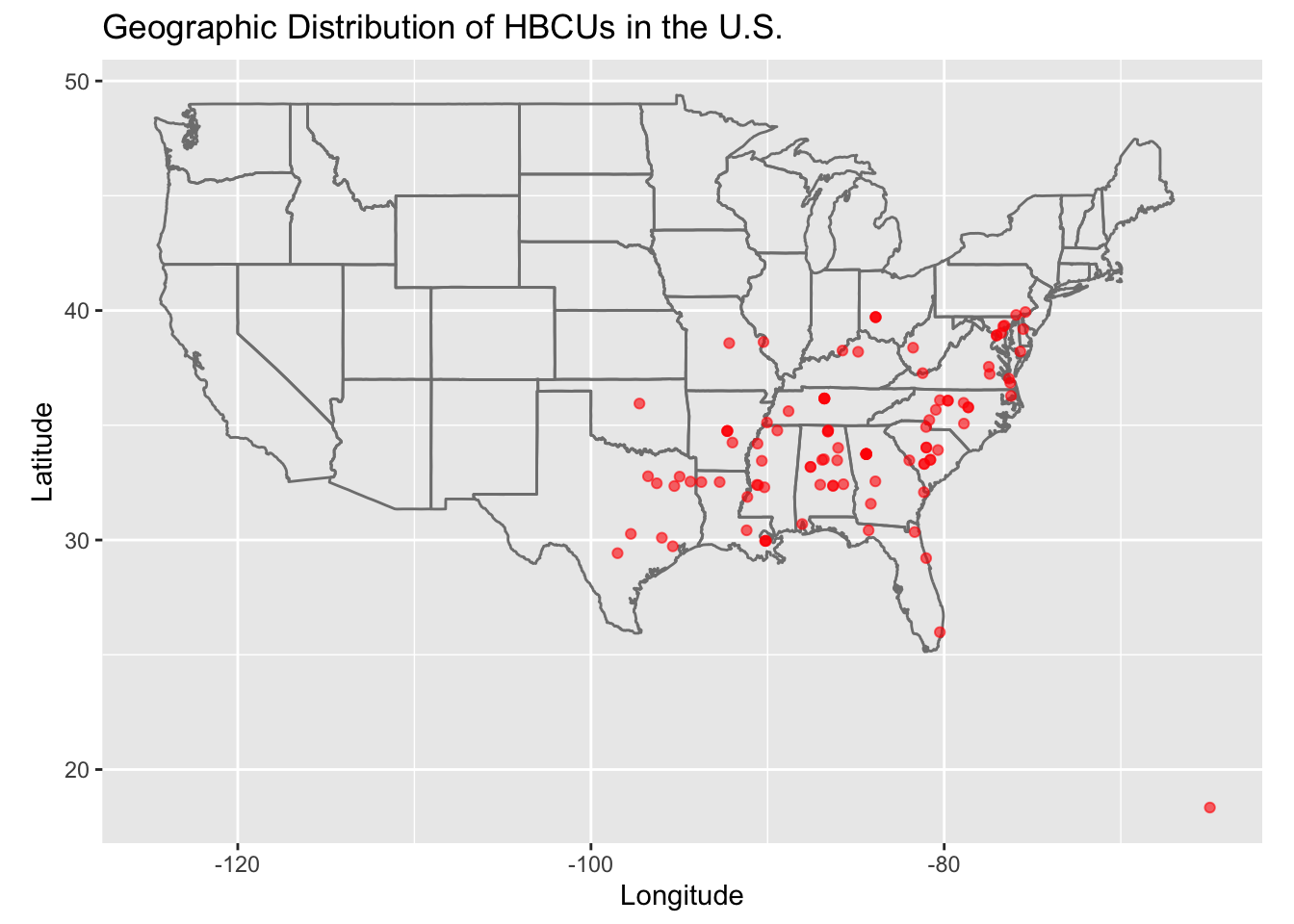
Step 6: Geographic Distribution

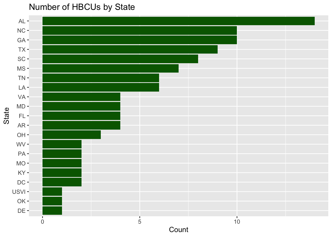
HBCUs by state

hbcu %>%
  count(state, sort = TRUE)

# A tibble: 21 × 2
   state     n
   <fct> <int>
 1 AL       14
 2 GA       10
 3 NC       10
 4 TX        9
 5 SC        8
 6 MS        7
 7 LA        6
 8 TN        6
 9 AR        4
10 FL        4
# ℹ 11 more rows

Basic visualization of HBCUs by state

hbcu %>%
  count(state) %>%
  ggplot(aes(x = reorder(state, n), y = n)) +
  geom_col(fill = "darkgreen") +
  coord_flip() +
  labs(
    title = "Number of HBCUs by State",
    x = "State",
    y = "Count"
  )

Step 7: Mapping

#install.packages("maps", repos = "http://cran.us.r-project.org")
library(maps)

hbcu %>%
  ggplot(aes(x = lon, y = lat)) +
  borders("state") +
  geom_point(color = "red", alpha = 0.6) +
  coord_fixed(1.3) +
  labs(
    title = "Geographic Distribution of HBCUs in the U.S.",
    x = "Longitude",
    y = "Latitude"
  )

Case Study: Data on State School Districts

Step 1: Load the libraries

library(dplyr)
library(readr)
library(stringr)
library(janitor)

Step 2: Load the data

district <- read.csv("https://github.com/quant-shop/intro-comp-educ-soc/blob/main/data/state-district-data.csv")
# district <- read.csv("../data/state-district-data.csv")

Step 3: Clean the data

district_clean <- district %>%
  clean_names() %>%
  mutate(across(everything(), ~na_if(., "–"))) %>%
  mutate(across(everything(), ~na_if(., "†"))) %>%
  mutate(across(where(is.character), ~str_trim(.))) %>%
  
  # Convert numeric-like columns
  mutate(across(
    contains("students") | contains("teachers") | contains("enrollment") | contains("ratio"),
    ~parse_number(.)
  ))

Step 4: Feature engineering

We can create variables that answer educational questions.

str(district_clean)

'data.frame':   2614 obs. of  1 variable:
 $ x_doctype_html: chr  "<html" "lang=en" "" "data-color-mode=auto data-light-theme=light data-dark-theme=dark" ...

# what kinds of questions might you answer with this data set?